Why vortex method?
Vortex is probably the most important kinetic behavior of fluid. Shear instability leads to concentrated vortices, baroclinic torque gives rise to vortex rings. Using vorticity equation as the prognostic discretized equation enjoys some numerical advantages. Vorticity is advected, twisted and stretched by velocity field which is induced by vorticity itself. Such nonlinear process leads to thin vortex filaments, which is hard to be captured without numerical oscillation. If we use vorticity equation as the prognostic equation, those intricate tracer advection schemes could be imposed on vorticity directly, and numerical oscillation and dispersion caused by vortex filaments could be greatly reduced.
The extension of traditional 2D vortex method to 3D proves difficult, for we now have a strange vector Poisson equation to invert velocity from vorticity. The velocity non-divergent condition is now implicit and serves as a constraint for the vector Poisson equation, preventing the direct application of popular fast solvers. To deal with this, we derived a simple and efficient multigrid Poisson solver and its fast convergence rate has been analytically proved.
Discretization
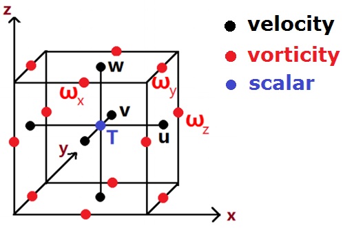
The model utilized staggered MAC grid, with scalar defined at cell center, velocity at cell surfaces, and vorticity at cell edges.
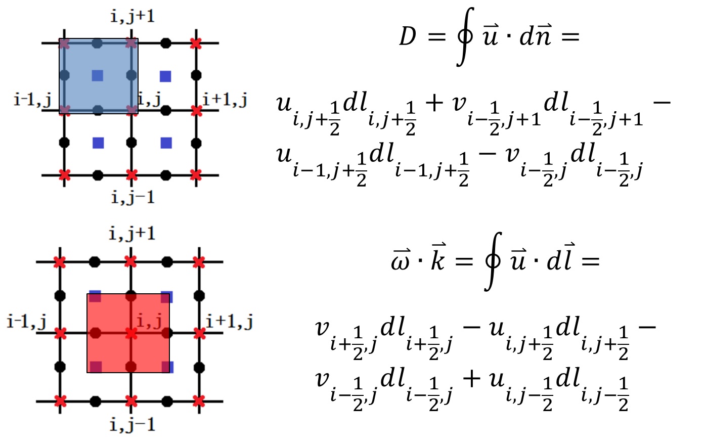
Vorticity is defined with circulation dividing a finite area, and divergence is defined as net mass flux dividing a finite volume.
With this, the discrete analog of ![]() is preserved (Bertagnoliio et al., 1997). It is useful in preserving a divergence free vorticity tendency, and therefore divergence free velocity during inversion.
is preserved (Bertagnoliio et al., 1997). It is useful in preserving a divergence free vorticity tendency, and therefore divergence free velocity during inversion.
 |
 |
| Variables on a staggered grid | Definition of divergence and vorticity |
Vorticity equation
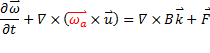
We write vorticity equation in curl form, in order to guarantee a divergence free vorticity tendency. Expanding each component of vorticity equation, we are surprised to find only 2 kinds of partial differentials exist in each equation.
Advection and twisting
High order finite volume method may not be economic in 3D, but is affordable now in this 2D case. We use fifth order WENO (Weighted Essentially Non-Oscillatory, Jiang et al., 1996) scheme on non-uniform grid. Gaussian integration points value are reconstructed in the same way for advection and twisting terms, in order to guarantee no divergence of vorticity.
![]()
![]()
![]()
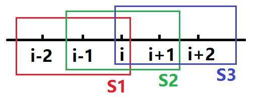 |
| WENO 5 stencils |
Diffusion
Diffusion term is discretized using vorticity cell averaged value as point value to calculate line integration, and has second order spatial accuracy.
![]()
Time Stepping
We use 3rd order TVD Runge-Kutta (Shu, 1998) to do time stepping. In each sub-step, the increment of advection-twisting and diffusion terms are summed. In fact, I plan to change this into operator splitting scheme.
![]()
![]()
![]()
Poisson equation
The Poisson equation is simply a vector analysis relation between vorticity and velocity, implicitly containing the velocity divergence free condition.
We parabolize the elliptic equation by adding a psudo-tendency term, and form the classical Jacobi iteration method. This is similar to the diffusion step of vorticity equation.
There are hardly any modern Poisson solvers that could hold the implicit divergence free condition, so they don’t help much. We analyzed the two major drawbacks of Jacobi iteration, and proposed our acceleration scheme.
- It has a notorious low convergence rate for long wave error.
--- Multigrid method
- Its psudo-time step is small, especially for refined grid area like boundary layer.
--- variable time step method
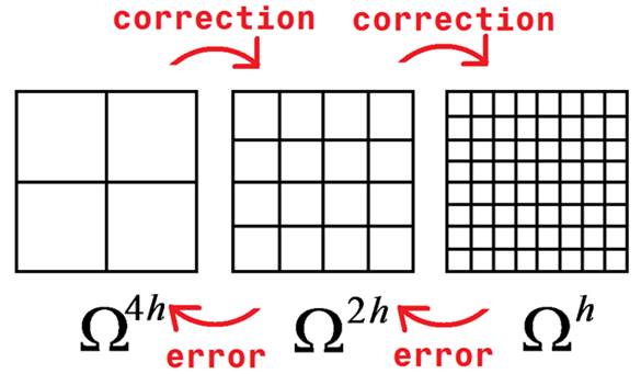
Multigrid method
Jacobi iteration can be viewed as smoothing the error (![]() ) over and over again until it diminishes to a low enough level.
) over and over again until it diminishes to a low enough level. ![]() damps short waves far more efficiently than long waves. If the grid is coarsened, a long wave error looks like a short wave error and could be easily eliminated. The key lies in designing a pair transfer operators between coarser and finer grids, in order to separate long and short waves clearly.
damps short waves far more efficiently than long waves. If the grid is coarsened, a long wave error looks like a short wave error and could be easily eliminated. The key lies in designing a pair transfer operators between coarser and finer grids, in order to separate long and short waves clearly.
The sequence of transporting the error is important. Here we adopt “V cycle”, with only one stroke from fine to coarse and back in each cycle. We first iterate a few times in the finest grid which is also the ordinary computational grid, find the error, and “restrict” the error to coarser grid. The error is all the way transported to the coarsest level, where we get the correction and is “prolongateded” down to the finest grid.
 |
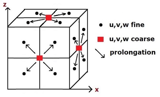 |
| a simple multigrid procedure | prolongation of velocity: from coarse to fine |
The restriction operator (from the fine to co arse) could be standard polynomial interpolation, but the prolongation operator (from coarse to fine) should be divergence-free and is thus our major concern. It means cutting a non-divergent cube into 8 non-divergent small cubes. This would be possible if the mass flux ratio on each face of the large cube is “inherited” by small cubes. Firstly, we split the face mass flux into two identical values. Secondly, we set the mass flux on newly-cut cross section with linear interpolation.
The only tunable parameters are iteration numbers on each level of grid. There should be enough iteration to damp short waves effectively in both restriction and prolongation operators, so as to avoid aliasing error during sampling.
The convergence rate estimate for monochromatic wave will be introduced in the document. We can also prove that the three component of vector Poisson equation is decoupled in this multigrid method.
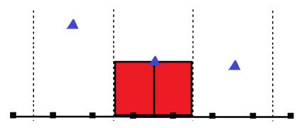 |
| a conservative split of velocity flux |
Flexible psudo-time step method
Jacobi iteration of elliptic equation is almost equivalent to the explicit scheme of parabolic equation, with a stability limit of (pseudo-) time step:
![]()
On the other hand, we usually refine the grid where the gradient of variables is large, take boundary layer for example. The small ![]() in boundary layer severely limits
in boundary layer severely limits ![]() . To deal with this, we have two steps.
. To deal with this, we have two steps.
Firstly, advance the unrefined region with the normal one time step, and advance the refined region with half the time step. Secondly, advance another half time step of refined region. Noticing that this procedure uses vorticity ![]() defined on the interface line of fined and refine region. We simply set:
defined on the interface line of fined and refine region. We simply set:
![]()
In this way, the velocity is guaranteed divergence free. Although the “time accuracy” drops below first order. It is of no concern to our elliptic solver which converges to a steady state, but may not be applicable to a parabolic equation which has unsteady solution. That’s why we don’t use this scheme in vorticity diffusion equation, and the equally severe time step constraint there inherently limits the model time step.
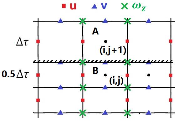 |
| The interface between the coarse and fine grid |